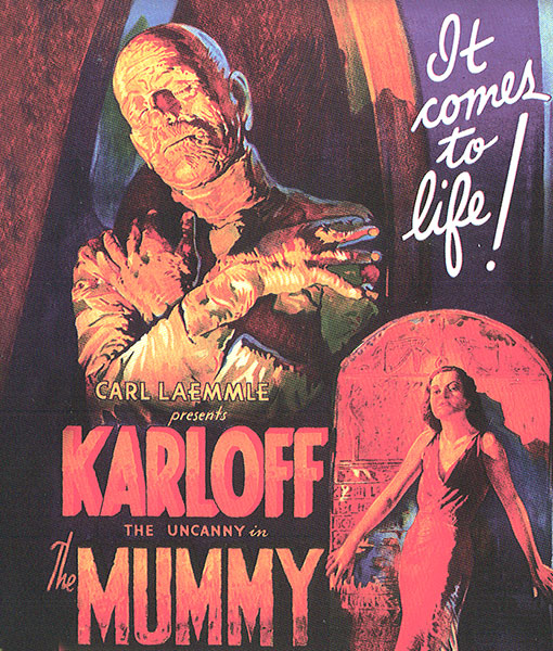
I’m thinking about Ancient Egypt for two reasons. For one thing, having seen the King Tut show , I’m thinking of bringing the mummy of Amenhotep into my novel, Jim and the Flims.
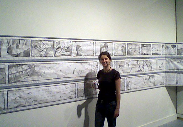
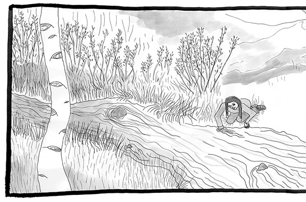
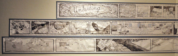
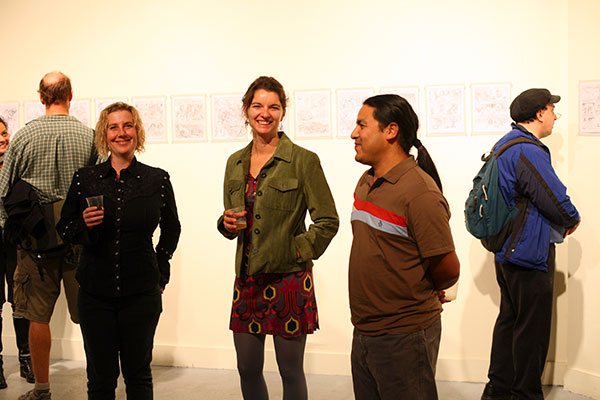
And for another, I enjoyed my daughter Isabel’s re-invention of hieroglyphics in some of the panels of her graphic novel Unfurling . I’ll reproduce a couple more images from Isabel’s graphic novel today—if you’re in the San Francisco area, you can still go see the show this month—see Isabel’s Unfurling page for more info.
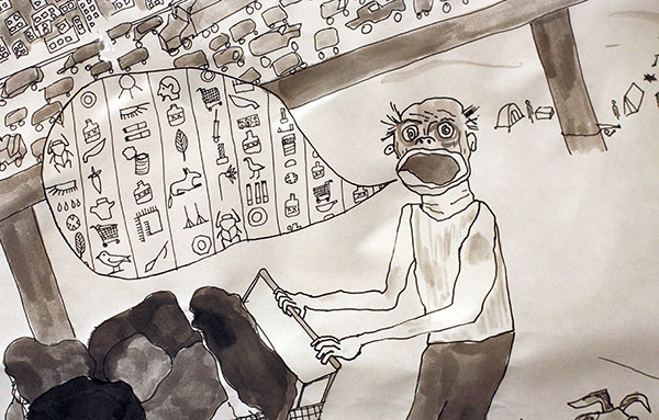
Several years ago, I gave Isabel a book on hieroglyphics, and she eventually came up with the brilliant notion of using a form of heiroglphyics as the native tongue of the restless street-people known as tweakers. (One of her friends suggested the language might be called Tweakenese.)
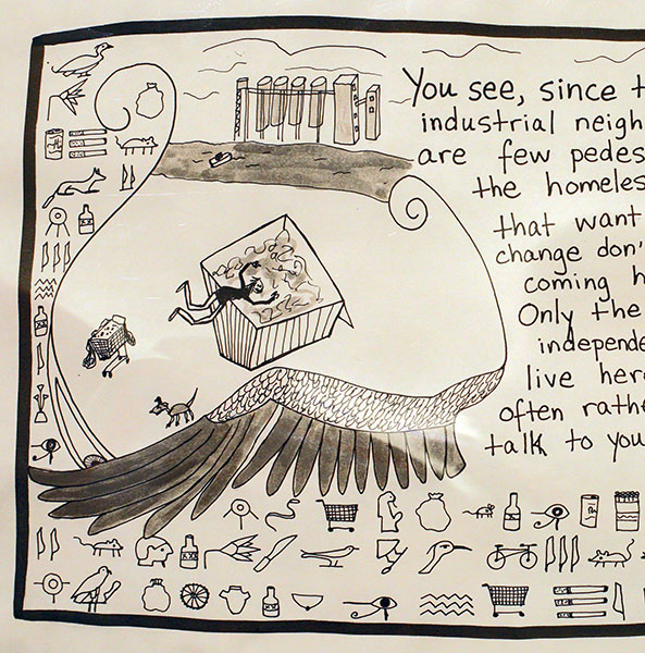
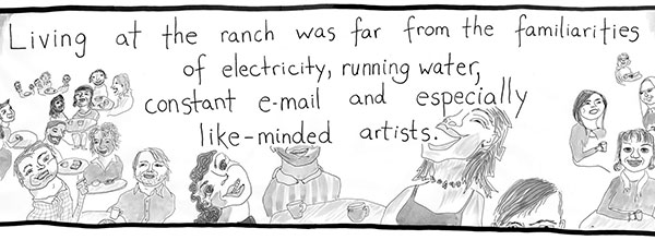
I love that there are glyphs for cigarettes and for shopping carts. And only a few different glyphs, really. When you look at ancient Egyptian hieroglyphics, it’s like they’re always talking about the same dozen or so things.
I’ve been gleaning more info about Egyptian notions of the afterlife—which I’d calling Flimsy in my novel—and I’ll reproduce some of it here, mostly edited from the Afterlife section of the Wikipedia article on Ancient Egyptian religion.
The ancient Egyptians believed that humans possessed a ka, or life-force, which left the body at the point of death. Even after death, the ka needed offerings of food, whose spiritual essence it could still consume. The ka might be thought of as simple existence or the bare notion of “I am.”

Each person also had a ba, the individual personality—what we might call software. Unlike the ka, the ba by default remained attached to the body after death. Egyptian funeral rituals were intended to release the ba from the body so that it could move freely. After being freed, the ba was believed to return to its mummified body each night to receive new life. Thus the state of the tomb and the mummy were important for the survival of both ka and ba.
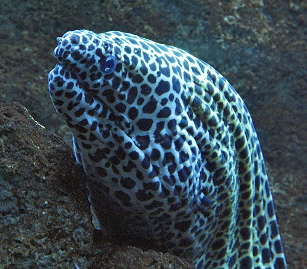
[Image taken from a blog post by a programmer named Xaprb.]
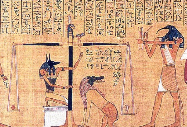
Once the ka was free to roam, its goal was to unite with the ba to form a complete soul, called an akh. In order to achieve this, the ba had to pass a judgment known as the Weighing of the Heart, where the jackal-headed god Anubis weighed the heart of the deceased against a feather (which symbolized Maat, the divine principle of fairness and order). The ibis-headed Thoth took notes.
If the heart was heavy, the ba was destroyed by the crocodile-headed demon Ammut, also known as the gobbler. Otherwise the ba united with the ka to form an akh. And then, by the way, you’d want to make sure that the gods gave you back your heart.
Specific beliefs about the activities of the akh varied. The vindicated dead were said to dwell in Osiris’ kingdom, a lush and pleasant land believed to exist somewhere beyond the western horizon, and kings were said to travel with Ra the sun-god in his boat that glides across the sky every day.
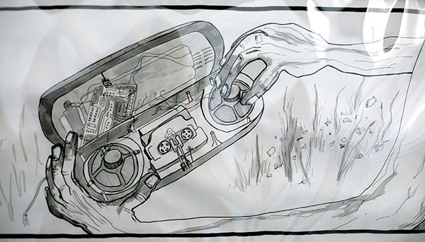
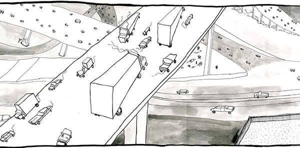
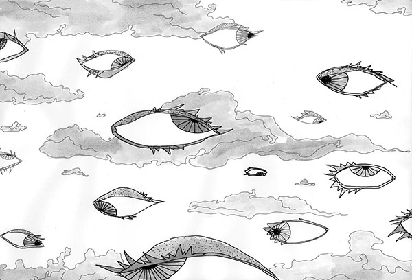
[This image is another detail from Unfurling again…I like the SF feel of it. The gnarled fingers tinkering with the broken hi-tech artifact.]
There was also a notion that an akh could also travel in the world of the living and magically affect events.

On a completely different topic, I saw Devo play their whole first album live at the Regency ballroom (about the size of the Fillmore) in San Francisco last week. Here’s a YouTube video that a guy standing in front of me made with his cell phone, it’s of their superficially non-PC (but, at a deeper level, rather empathetic) song “Mongoloid”.
It was great to see Devo come out and kick butt with their music. They’re old, but they’ve gotten very tight and extreme. We had a great cheer session. “Are we not men???” the bass player would bellow, and we’d roar back, “We are Devo!!!” My favorite moment was when they took an instrumental break during this strong, and were just shredding the music.
I still recall how liberating I found that first Devo album. Like the Ramones, Devo made me want to write science-fiction in a certain kind of way. Extreme, rocking, in your face, dadaistic, and easy to absorb.
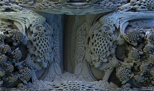
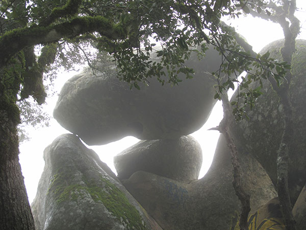
[“Cave of the Lost Secrets” image by Daniel White.]
Yet another topic: the Mandelbulb, that is the long-sought three-dimensional versions of the Mandelbrot fractal, which I blogged about before in my post, “In Search of the Mandelbulb.” Daniel White has just posted a very nice summary of his work on the Mandelbulb.